Run ANOVA in Excel

Introduction to ANOVA in Excel

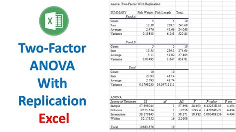
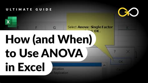
Analysis of Variance (ANOVA) is a statistical technique used to compare means of three or more samples to find out if at least one of the means is different. In Microsoft Excel, you can run ANOVA using the Analysis ToolPak add-in. This add-in provides a variety of statistical tools, including ANOVA.

Enabling the Analysis ToolPak

To run ANOVA in Excel, you first need to ensure that the Analysis ToolPak is enabled. Here’s how you can do it:

• Go to the “File” tab in Excel.
• Click on “Options” and then select “Add-ins” from the left sidebar.
• In the “Manage” dropdown at the bottom, select “Excel Add-ins” and click “Go”.
• Check the box next to “Analysis ToolPak” and click “OK”. If you don’t see it in the list, you might need to browse for it or install it if it’s not available.

Preparing Your Data

Before running ANOVA, your data should be organized in a specific way. Typically, each sample should be in a separate column, and the data should not contain any blank cells. Ensure your data is clean and ready for analysis.

Running ANOVA

Here’s a step-by-step guide to running ANOVA in Excel:

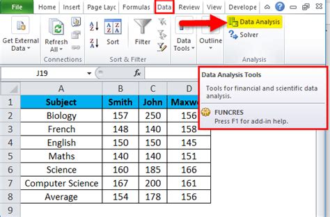
• Go to the “Data” tab in Excel.
• Click on “Data Analysis” in the “Analysis” group. If you don’t see this button, it might be because the Analysis ToolPak is not enabled.
• In the “Data Analysis” dialog box, scroll down and select “Anova: Single Factor” and click “OK”. This is the most common type of ANOVA for comparing multiple groups.
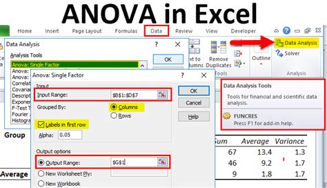
• In the “Anova: Single Factor” dialog box, you need to select the range of your data. Click in the “Input Range” box and then select your data, including headers if you have them.
• Choose whether your data is in columns or rows. If each sample is in a separate column, select “Columns”. If each row represents a separate observation, you might need to select “Rows”, but this is less common for ANOVA setup.
• If you have labels in the first row (headers), check the “Labels in first row” box.
• Choose an output range or select to put the output in a new worksheet by clicking on the appropriate radio button.
• Click “OK” to run the ANOVA.

Interpreting ANOVA Results

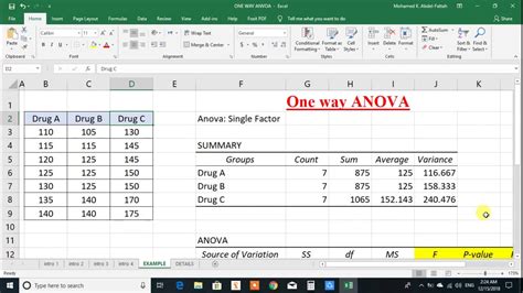
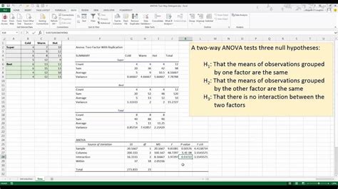
After running ANOVA, Excel will provide you with a table that includes several statistical values. The key values to look at are:

• SS (Sum of Squares): This is a measure of the variation in your data.
• df (Degrees of Freedom): This is related to the number of observations and groups you have.
• MS (Mean Square): This is the average of the SS, adjusted for the df.
• F: This is the F-statistic, which is the ratio of the MS between groups to the MS within groups.
• P-value: This tells you the probability of observing your results (or more extreme) assuming that there is no real difference between the groups. Typically, if the P-value is less than 0.05, you reject the null hypothesis that all means are equal.

The F-statistic and P-value are crucial for determining whether there is a significant difference between the means of your samples.

Source of Variation	SS	df	MS	F	P-value
Between Groups	X	Y	Z	A	B
Within Groups	X	Y	Z
Total	X	Y

📝 Note: Always ensure your data meets the assumptions of ANOVA, such as normality and equal variances, before interpreting the results.

To further understand the differences between specific groups if the ANOVA test indicates a significant difference, you might need to conduct post-hoc tests like Tukey’s HSD.

Post-Hoc Tests

Post-hoc tests are used after ANOVA to determine which specific groups are different from each other. Excel does not directly provide post-hoc tests within the Analysis ToolPak, but you can use other statistical software or calculate them manually with formulas.

Summary of Key Points

Running ANOVA in Excel involves enabling the Analysis ToolPak, preparing your data, selecting the appropriate ANOVA type, and interpreting the results based on the F-statistic and P-value. Remember to check the assumptions of ANOVA and consider post-hoc tests if you find significant differences between your groups.

The process of analyzing data with ANOVA in Excel is straightforward once you have your data organized and the Analysis ToolPak enabled. It provides a powerful tool for comparing means across multiple groups, helping you understand if there are statistically significant differences.